Data With Geometry

This notebook demonstrates how we can load the geometry of geographical locations when we load the data associated with them just by adding the with_geoemetry=True flag to a call to censusdis.data.download_detail.

This is a nice powerful feature because it saves us the time of loading data and maps separately and dealing with the not-quite-matching column names we have to join them on. Setting this one flag saves us all that effort.

Imports and configuration

[1]:

# So we can run from within the censusdis project and find the packages we need.
import os
import sys

sys.path.append(
    os.path.join(os.path.abspath(os.path.join(os.path.curdir, os.path.pardir)))
)

[2]:

import os

import geopandas as gpd
import matplotlib.pyplot as plt

from typing import Optional

import censusdis.data as ced
import censusdis.maps as cem
from censusdis.states import ALL_STATES_AND_DC, STATE_NAMES_FROM_IDS, STATE_GA

[3]:

SHAPEFILE_ROOT = os.path.join(os.environ["HOME"], "data", "shapefiles")

# Make sure it is there.
os.makedirs(SHAPEFILE_ROOT, exist_ok=True)

What dataset and variables?

[4]:

DATASET = "acs/acs5"
YEAR = 2020

[5]:

# This is a census variable for median household income.
# See https://api.census.gov/data/2020/acs/acs5/variables/B19013_001E.html
MEDIAN_HOUSEHOLD_INCOME_VARIABLE = "B19013_001E"

[6]:

VARIABLES = ["NAME", MEDIAN_HOUSEHOLD_INCOME_VARIABLE]

[7]:

MISSING_VALUE = -666666666

Shapefile reader

[8]:

reader = cem.ShapeReader(SHAPEFILE_ROOT, year=YEAR)
ced.set_shapefile_path(SHAPEFILE_ROOT)

[9]:

gdf_state_bounds = reader.read_cb_shapefile("us", "state")
gdf_state_bounds = gdf_state_bounds[gdf_state_bounds["STATEFP"].isin(ALL_STATES_AND_DC)]

Function to drop missing values

[10]:

CENSUS_MISSING_VALUE = -666666666


def drop_missing_mhi(gdf: gpd.GeoDataFrame) -> gpd.GeoDataFrame:
    return gdf[gdf[MEDIAN_HOUSHOLD_INCOME_VARIABLE] != CENSUS_MISSING_VALUE]

Plot function

[34]:

plt.rcParams["figure.figsize"] = (18, 8)


def plot_map(
    gdf: gpd.GeoDataFrame,
    geo: str,
    *,
    gdf_bounds: Optional[gpd.GeoDataFrame] = None,
    bounds_color: str = "white",
    max_income: float = 200_000.0,
):
    if gdf_bounds is None:
        gdf_bounds = gdf

    ax = cem.plot_us(gdf_bounds, color="lightgray")

    ax = cem.plot_us(
        gdf,
        MEDIAN_HOUSHOLD_INCOME_VARIABLE,
        cmap="autumn",
        legend=True,
        vmin=0.0,
        vmax=max_income,
        ax=ax,
    )

    ax = cem.plot_us_boundary(gdf_bounds, edgecolor=bounds_color, linewidth=0.5, ax=ax)

    ax.set_title(f"{YEAR} Median Household Income by {geo.title()}")

    ax.axis("off")

    plt.savefig(os.path.join(os.environ["HOME"], "tmp", "plot.png"))

Query with geography

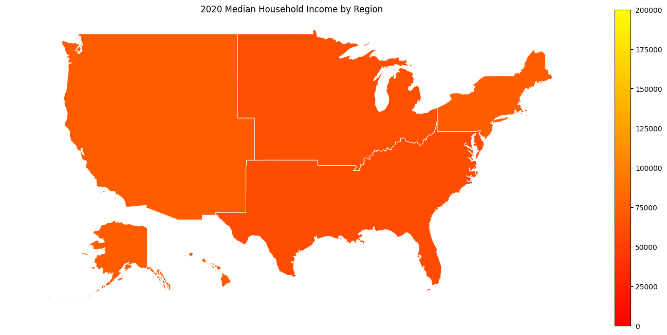
Region

[12]:

gdf_region = ced.download_detail(
    DATASET, YEAR, VARIABLES, region="*", with_geometry=True
)

[13]:

plot_map(gdf_region, "region")

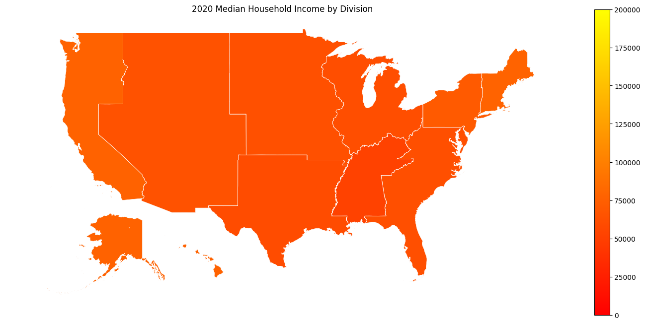
../_images/nb_Data_With_Geometry_21_0.png

Division

[14]:

gdf_division = ced.download_detail(
    DATASET, YEAR, VARIABLES, division="*", with_geometry=True
)

[15]:

plot_map(gdf_division, "division")

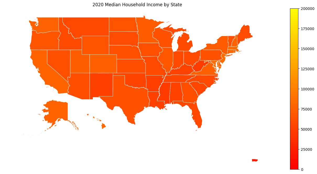
../_images/nb_Data_With_Geometry_24_0.png

State

[16]:

gdf_state = ced.download_detail(DATASET, YEAR, VARIABLES, state="*", with_geometry=True)

[17]:

plot_map(gdf_state, "state")

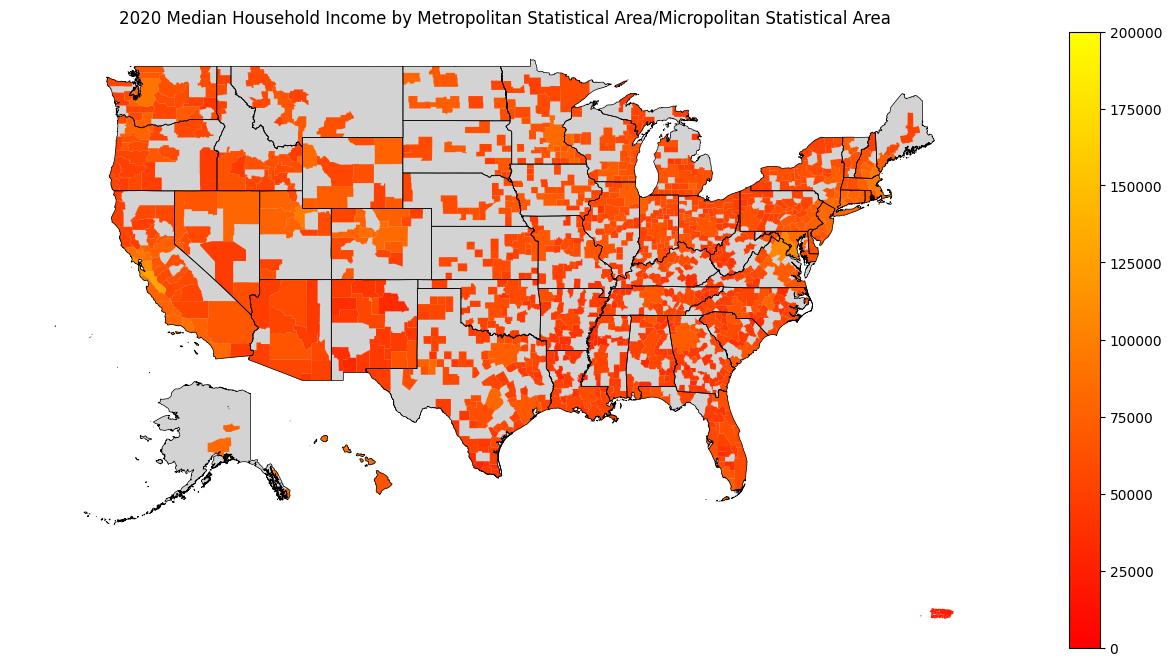
../_images/nb_Data_With_Geometry_27_0.png

CBSA

[18]:

gdf_cbsa = ced.download_detail(
    DATASET,
    YEAR,
    VARIABLES,
    metropolitan_statistical_area_micropolitan_statistical_area="*",
    with_geometry=True,
)

[19]:

plot_map(
    gdf_cbsa,
    "metropolitan statistical area/micropolitan statistical area",
    gdf_bounds=gdf_state_bounds,
    bounds_color="black",
)

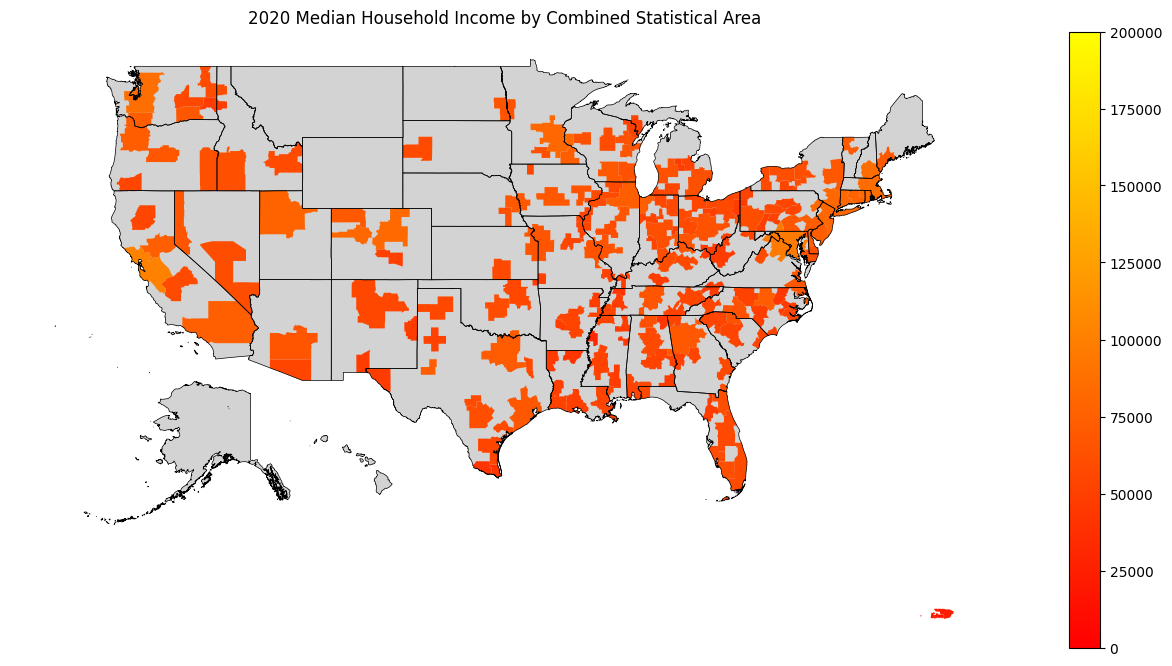
../_images/nb_Data_With_Geometry_30_0.png

CSA

[20]:

gdf_csa = ced.download_detail(
    DATASET, YEAR, VARIABLES, combined_statistical_area="*", with_geometry=True
)

[21]:

plot_map(
    gdf_csa,
    "combined statistical area",
    gdf_bounds=gdf_state_bounds,
    bounds_color="black",
)

../_images/nb_Data_With_Geometry_33_0.png

County

[22]:

gdf_county = ced.download_detail(
    DATASET, YEAR, VARIABLES, state="*", county="*", with_geometry=True
)

[23]:

plot_map(gdf_county, "county", gdf_bounds=gdf_state_bounds)

../_images/nb_Data_With_Geometry_36_0.png

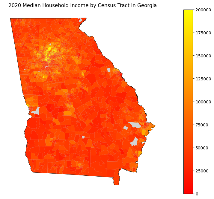
Census Tract

[24]:

STATE = STATE_GA

[25]:

gdf_tract = ced.download_detail(
    DATASET, YEAR, VARIABLES, state=STATE, tract="*", with_geometry=True
)

gdf_tract = drop_missing_mhi(gdf_tract)

[26]:

plot_map(
    gdf_tract,
    f"census tract in {STATE_NAMES_FROM_IDS[STATE]}",
    gdf_bounds=gdf_state_bounds[gdf_state_bounds["STATEFP"] == STATE],
    bounds_color="black",
)

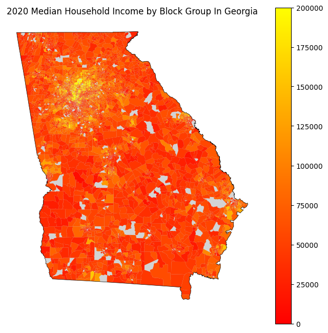
../_images/nb_Data_With_Geometry_40_0.png

Block Group

[27]:

gdf_bg = ced.download_detail(
    DATASET, YEAR, VARIABLES, state=STATE, block_group="*", with_geometry=True
)

[28]:

gdf_bg = drop_missing_mhi(gdf_bg)

[36]:

plt.rcParams["figure.figsize"] = (8, 8)

plot_map(
    gdf_bg,
    f"block group in {STATE_NAMES_FROM_IDS[STATE]}",
    gdf_bounds=gdf_state_bounds[gdf_state_bounds["STATEFP"] == STATE],
    bounds_color="black",
)

../_images/nb_Data_With_Geometry_44_0.png

[ ]: