Data With Geometry

This notebook demonstrates how we can load the geometry of geographical locations when we load the data associated with them just by adding the with_geoemetry=True flag to a call to censusdis.data.download.

This is a nice powerful feature because it saves us the time of loading data and maps separately and dealing with the not-quite-matching column names we have to join them on. Setting this one flag saves us all that effort.

Imports and configuration

[1]:

import os

import geopandas as gpd
import matplotlib.pyplot as plt

from typing import Optional

import censusdis.data as ced
import censusdis.maps as cem
import censusdis.values as cev
from censusdis import states

What dataset and variables?

[2]:

DATASET = "acs/acs5"
YEAR = 2020

[3]:

# This is a census variable for median household income.
# See https://api.census.gov/data/2020/acs/acs5/variables/B19013_001E.html
MEDIAN_HOUSEHOLD_INCOME_VARIABLE = "B19013_001E"

[4]:

VARIABLES = ["NAME", MEDIAN_HOUSEHOLD_INCOME_VARIABLE]

Shapefile reader

[5]:

reader = cem.ShapeReader(year=YEAR)

[6]:

gdf_state_bounds = reader.read_cb_shapefile("us", "state")
gdf_state_bounds = gdf_state_bounds[
    gdf_state_bounds["STATEFP"].isin(states.ALL_STATES_AND_DC)
]

Plot function

[7]:

plt.rcParams["figure.figsize"] = (18, 8)


def plot_map(
    gdf: gpd.GeoDataFrame,
    geo: str,
    *,
    gdf_bounds: Optional[gpd.GeoDataFrame] = None,
    bounds_color: str = "white",
    max_income: float = 200_000.0,
    **kwargs,
):
    """Plot a map."""
    if gdf_bounds is None:
        gdf_bounds = gdf

    ax = cem.plot_us(gdf_bounds, color="lightgray")

    ax = cem.plot_us(
        gdf,
        MEDIAN_HOUSEHOLD_INCOME_VARIABLE,
        cmap="autumn",
        edgecolor="darkgray",
        legend=True,
        vmin=0.0,
        vmax=max_income,
        ax=ax,
        **kwargs,
    )

    ax = cem.plot_us_boundary(gdf_bounds, edgecolor=bounds_color, linewidth=0.5, ax=ax)

    ax.set_title(f"{YEAR} Median Household Income by {geo.title()}")

    ax.axis("off")

Query with geography

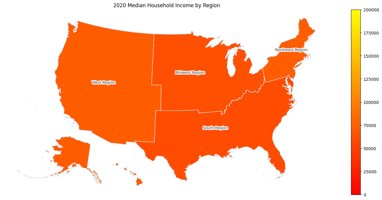
Region

[8]:

gdf_region = ced.download(DATASET, YEAR, VARIABLES, region="*", with_geometry=True)

[9]:

plot_map(gdf_region, "region", geo_label="NAME")

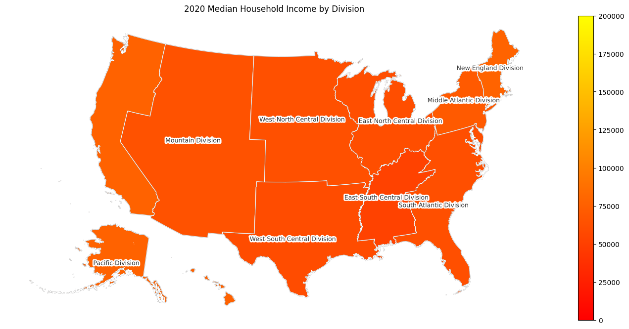
../_images/nb_Data_With_Geometry_16_0.png

Division

[10]:

gdf_division = ced.download(DATASET, YEAR, VARIABLES, division="*", with_geometry=True)

[11]:

plot_map(gdf_division, "division", geo_label=gdf_division["NAME"])

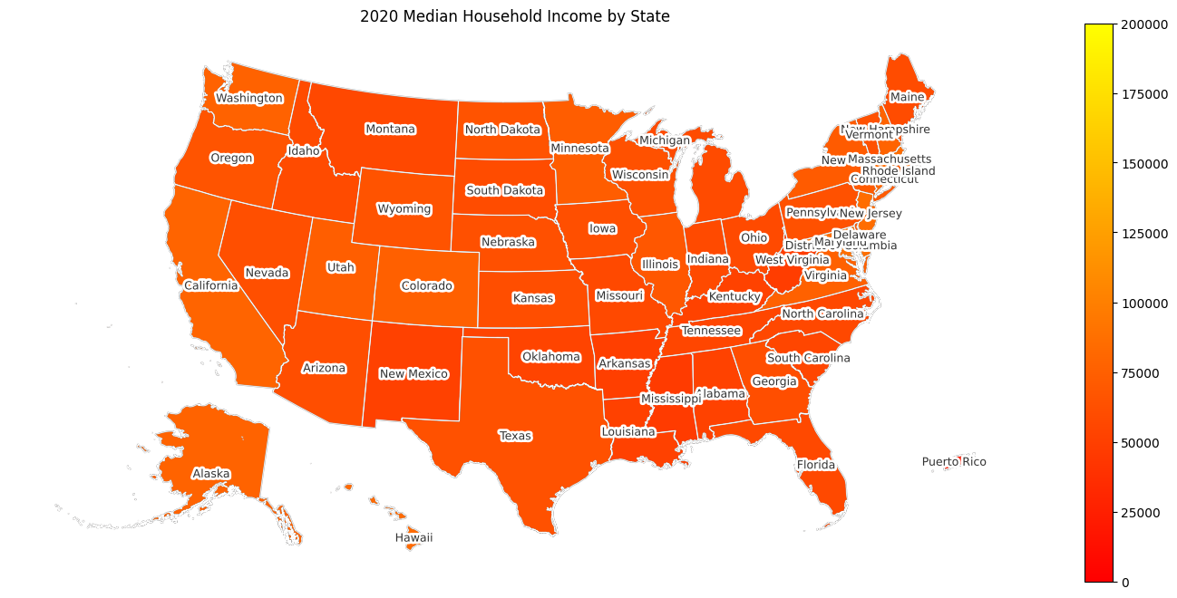
../_images/nb_Data_With_Geometry_19_0.png

State

[12]:

gdf_state = ced.download(DATASET, YEAR, VARIABLES, state="*", with_geometry=True)

[13]:

plot_map(gdf_state, "state", geo_label="NAME")

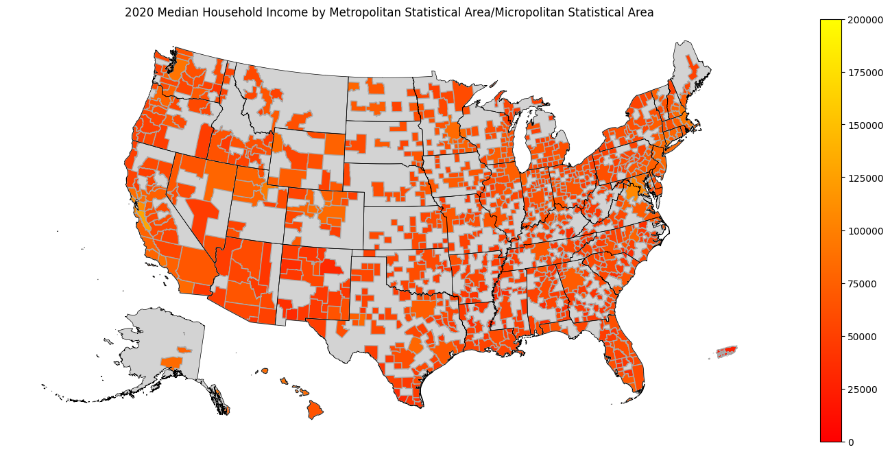
../_images/nb_Data_With_Geometry_22_0.png

CBSA

[14]:

gdf_cbsa = ced.download(
    DATASET,
    YEAR,
    VARIABLES,
    metropolitan_statistical_area_micropolitan_statistical_area="*",
    with_geometry=True,
)

[15]:

plot_map(
    gdf_cbsa,
    "metropolitan statistical area/micropolitan statistical area",
    gdf_bounds=gdf_state_bounds,
    bounds_color="black",
)

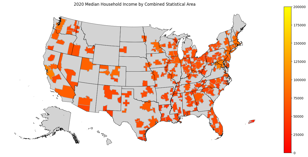
../_images/nb_Data_With_Geometry_25_0.png

CSA

[16]:

gdf_csa = ced.download(
    DATASET, YEAR, VARIABLES, combined_statistical_area="*", with_geometry=True
)

[17]:

plot_map(
    gdf_csa,
    "combined statistical area",
    gdf_bounds=gdf_state_bounds,
    bounds_color="black",
)

../_images/nb_Data_With_Geometry_28_0.png

County

[18]:

gdf_county = ced.download(
    DATASET, YEAR, VARIABLES, state="*", county="*", with_geometry=True
)

[19]:

plot_map(gdf_county, "county", gdf_bounds=gdf_state_bounds)

../_images/nb_Data_With_Geometry_31_0.png

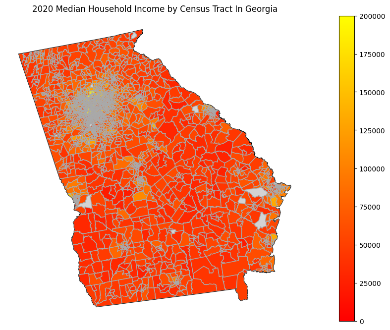
Census Tract

[20]:

STATE = states.GA

[21]:

gdf_tract = ced.download(
    DATASET,
    YEAR,
    VARIABLES,
    state=STATE,
    tract="*",
    with_geometry=True,
    set_to_nan=cev.ALL_SPECIAL_VALUES,
)

[22]:

plot_map(
    gdf_tract,
    f"census tract in {states.NAMES_FROM_IDS[STATE]}",
    gdf_bounds=gdf_state_bounds[gdf_state_bounds["STATEFP"] == STATE],
    bounds_color="black",
)

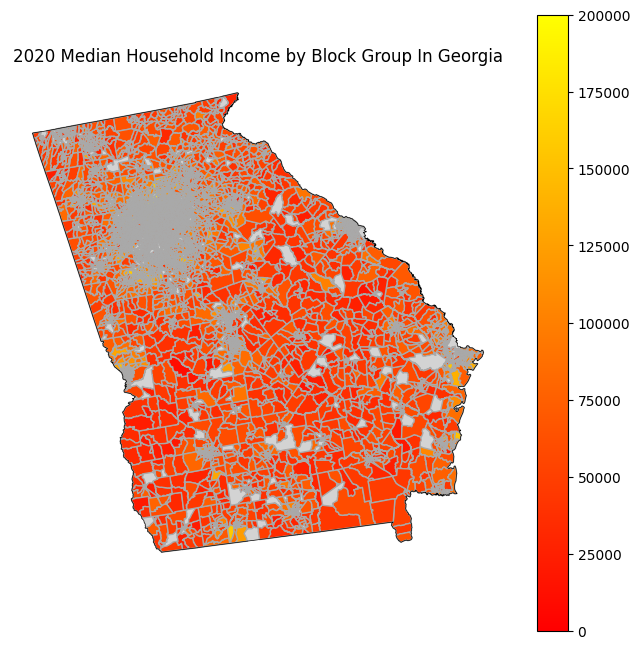
../_images/nb_Data_With_Geometry_35_0.png

Block Group

[23]:

gdf_bg = ced.download(
    DATASET,
    YEAR,
    VARIABLES,
    state=STATE,
    block_group="*",
    with_geometry=True,
    set_to_nan=cev.ALL_SPECIAL_VALUES,
)

[24]:

plt.rcParams["figure.figsize"] = (8, 8)

plot_map(
    gdf_bg,
    f"block group in {states.NAMES_FROM_IDS[STATE]}",
    gdf_bounds=gdf_state_bounds[gdf_state_bounds["STATEFP"] == STATE],
    bounds_color="black",
)

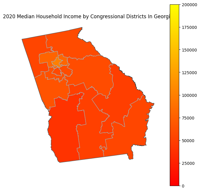
../_images/nb_Data_With_Geometry_38_0.png

Congressional District

[25]:

gdf_cd = ced.download(
    DATASET,
    YEAR,
    VARIABLES,
    state=STATE,
    congressional_district="*",
    with_geometry=True,
    set_to_nan=cev.ALL_SPECIAL_VALUES,
)

[26]:

plt.rcParams["figure.figsize"] = (8, 8)

plot_map(
    gdf_cd,
    f"congressional districts in {states.NAMES_FROM_IDS[STATE]}",
    gdf_bounds=gdf_state_bounds[gdf_state_bounds["STATEFP"] == STATE],
    bounds_color="black",
)

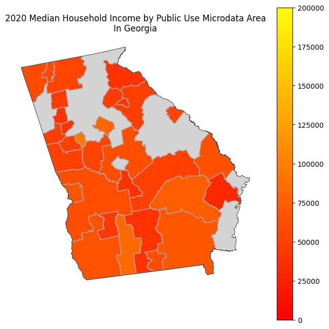
../_images/nb_Data_With_Geometry_41_0.png

Public Use Microdata Area

[27]:

gdf_puma = ced.download(
    DATASET,
    YEAR,
    VARIABLES,
    state=STATE,
    public_use_microdata_area="*",
    with_geometry=True,
    set_to_nan=cev.ALL_SPECIAL_VALUES,
)

[28]:

plt.rcParams["figure.figsize"] = (8, 8)

plot_map(
    gdf_puma,
    f"public use microdata area\nin {states.NAMES_FROM_IDS[STATE]}",
    gdf_bounds=gdf_state_bounds[gdf_state_bounds["STATEFP"] == STATE],
    bounds_color="black",
)

../_images/nb_Data_With_Geometry_44_0.png

[ ]: