SoMA DIS Demo
[1]:
# So we can run from within the censusdis project and find the packages we need.
import os
import sys

sys.path.append(
    os.path.join(os.path.abspath(os.path.join(os.path.curdir, os.path.pardir)))
)
Introduction
In this notebook, we will demonstrate how to use the `censusdis <https://github.com/vengroff/censusdis>`__ package to download some US Census data and then how to use the `divintseg <https://github.com/vengroff/divintseg>`__ package to compute some diversity and integration metrics.
In this example, we will look at US Census redistricting data from the towns of South Orange and Maplewood (collectively known as SoMa) in Essex County, NJ. We chose redistricting data because it has the demographic data we are interested in studying, including race and ethnicity.
Once you are familiar with the API and how to use it, you can easily experiment with similar analysis of the area where you live.
Environment Setup
We assume you are running this notebook in an environment where the necessary packages have been pip installed. You should be able to get everything you need with just
pip install censusdis
which will also install divintseg and various other dependencies.
Imports
We need to import out resistricting data API, some utilities for getting map data, and the `divintseg <https://github.com/vengroff/divintseg>`__ package that computes diversity and integration metrics, along with pandas for some basic data manipulation.
[2]:
import censusdis.data as ced
import censusdis.maps as cem

from censusdis.states import STATE_NJ
from censusdis.counties.new_jersey import ESSEX

import divintseg as dis

import pandas as pd
US Census API Key
The US Census API uses a key to identify callers. If you don’t already have a key, you can request one here. Please put your key into this cell before running the notebook.
For small queries like in this demo notebook, the API seems to work without a key, so you can leave it set to None, but for more serious work you will want to obtain a key.
[3]:
CENSUS_API_KEY = None
Basic Configuration
Year
US Cansus data is organized by the year it was collected. For the moment, we are interested in the year 2020.
[4]:
YEAR = 2020
Dataset
In any given year, the US Census publishes a wide variety of data, which comes in different collections called datasets. A dataset typically consists of a wide variety of data gathered at the same time using the same methodology.
The dataset we are interested in using is called the Decennial Census: Redistricting Data (PL 94-171).
In code is commonly known as dec/pl, which is how we will refer to it here.
[5]:
DATASET = "dec/pl"
Group
A group is a set of related variables within a dataset. Groups cover all kinds of topics. We are using 2020 dec/pl redistricting data, so the groups available are those summarized at https://api.census.gov/data/2020/dec/pl/groups.html. Notice how the URL just keeps buidling up as we go from year to dataset to group.
Don’t worry if nothing on that page means anything to you right now. We’ll explain it here.
If we choose P1, then the data is grouped purely based on race, not taking ethnicity into account at all. If we choose P2, then the data is first grouped by ethnicity, with people reporting Hispanic or Latino ethinicity put into one group regardless of their race. Everyone else is then divided into groups based on their race.
Thus, P2 has one group that P1 does not have, which is Hispanic or Latino of any race. In the P1 data set, people who are in the Hispanic or Latino group in P2 are instead classified into one of the race-based groups.
For more information, including additional options P3 and P4, see this additional documentation.
[6]:
GROUP = "P2"
Variables and Groups
The variables in many groups exist in tree-structured hierarchy. We can see the hierarchy for our group by looking at the labels in the second column of the table at https://api.census.gov/data/2020/dec/pl/groups/P2.html
We are most interested in the leaves of this tree, which are the populations of people that are not further subdivided. P2_002N is a leaf because the population that is Hispanic or Latino is not further subdivided. P2_003N is not a leaf, because it is further subdivided into P2_004N and P2_011N.
Luckily, we don’t have to read through the table of variables in the group and carefully keep track of what are leaves and what aren’t. Instead, as we will see when we download data, we can simply specify the group whose leaves we want data for as part of the ced.download call.
If we want to get the leaves explicitly and look at them, we can also do that.
[7]:
leaves = ced.variables.group_leaves(DATASET, YEAR, GROUP)
If you start looking the first ten or so fields up in in the table at https://api.census.gov/data/2020/dec/pl/groups/P2.html you should be able to convince yourself that we successfully found the leaves. Note that there are also annotation fields listed in the table, but the API we used skipped those by default.
[8]:
leaves[:10]
[8]:
['P2_002N',
 'P2_005N',
 'P2_006N',
 'P2_007N',
 'P2_008N',
 'P2_009N',
 'P2_010N',
 'P2_013N',
 'P2_014N',
 'P2_015N']
South Orange and Maplewood Tracts in Essex County, NJ
Now that we know what variables we are interested in, we want to get data for them from the towns of South Orange and Maplewood (collectively known as SoMa) in Essex County, NJ.
SoMa Tracts
We found the tracts that make up the two towns by looking at this map. We format them as strings using the convention of Census API, which is a six-digit string.
[9]:
tracts_soma = [f"{t:06}" for t in range(19000, 20000, 100)]
tracts_soma
[9]:
['019000',
 '019100',
 '019200',
 '019300',
 '019400',
 '019500',
 '019600',
 '019700',
 '019800',
 '019900']
SoMa Data Query
Now we can query the data. See the inline comments for descriptions of the various arguments we pass.
The return value will be a pd.DataFrame containing a row for each block (the resolution we specified). In order to make analysis of diversity and integration at various levels of geographic aggregation easier (e.g. using the divintseg package) the identifiers of all of the nested geographies from the state down to the block are included in each row. In this case that means we have columns for STATE, COUNTY, TRACT, BLOCK_GROUP, and BLOCK. After
these columns, we have one column for each of the demographic fields we asked for.
[10]:
df_soma = ced.download(
    # First we specify the dataset and year:
    DATASET,
    YEAR,
    # Next, the group of variables we want to get data for:
    leaves_of_group=GROUP,
    # Next come filters that constrain what data we
    # want to load, specified as keyword arguments.
    # The narrowest of these, which in our case is
    # block, specifies the level of aggregation. We
    # use block=* to indicate all blocks within the
    # tracts we have specified.
    state=STATE_NJ,
    county=ESSEX,
    tract=tracts_soma,
    block="*",
    # Finally, we put in our API key:
    api_key=CENSUS_API_KEY,
)
[11]:
df_soma
[11]:
| STATE | COUNTY | TRACT | BLOCK | P2_002N | P2_005N | P2_006N | P2_007N | P2_008N | P2_009N | ... | P2_062N | P2_063N | P2_064N | P2_066N | P2_067N | P2_068N | P2_069N | P2_070N | P2_071N | P2_073N | |
|---|---|---|---|---|---|---|---|---|---|---|---|---|---|---|---|---|---|---|---|---|---|
| 0 | 34 | 013 | 019400 | 1004 | 3 | 39 | 0 | 0 | 0 | 0 | ... | 0 | 0 | 0 | 0 | 0 | 0 | 0 | 0 | 0 | 0 |
| 1 | 34 | 013 | 019400 | 1005 | 7 | 78 | 8 | 0 | 1 | 0 | ... | 0 | 0 | 0 | 0 | 0 | 0 | 0 | 0 | 0 | 0 |
| 2 | 34 | 013 | 019400 | 1006 | 1 | 57 | 4 | 0 | 1 | 0 | ... | 0 | 0 | 0 | 0 | 0 | 0 | 0 | 0 | 0 | 0 |
| 3 | 34 | 013 | 019400 | 1007 | 1 | 9 | 4 | 0 | 8 | 0 | ... | 0 | 0 | 0 | 0 | 0 | 0 | 0 | 0 | 0 | 0 |
| 4 | 34 | 013 | 019400 | 1008 | 0 | 0 | 0 | 0 | 0 | 0 | ... | 0 | 0 | 0 | 0 | 0 | 0 | 0 | 0 | 0 | 0 |
| ... | ... | ... | ... | ... | ... | ... | ... | ... | ... | ... | ... | ... | ... | ... | ... | ... | ... | ... | ... | ... | ... |
| 512 | 34 | 013 | 019900 | 2007 | 3 | 113 | 3 | 0 | 6 | 0 | ... | 0 | 0 | 0 | 0 | 0 | 0 | 0 | 0 | 0 | 0 |
| 513 | 34 | 013 | 019900 | 2010 | 3 | 26 | 3 | 0 | 1 | 0 | ... | 0 | 0 | 0 | 0 | 0 | 0 | 0 | 0 | 0 | 0 |
| 514 | 34 | 013 | 019900 | 3001 | 2 | 70 | 0 | 0 | 0 | 0 | ... | 0 | 0 | 0 | 0 | 0 | 0 | 0 | 0 | 0 | 0 |
| 515 | 34 | 013 | 019900 | 3005 | 6 | 49 | 1 | 0 | 2 | 0 | ... | 0 | 0 | 0 | 0 | 0 | 0 | 0 | 0 | 0 | 0 |
| 516 | 34 | 013 | 019900 | 3008 | 4 | 66 | 0 | 0 | 1 | 1 | ... | 0 | 0 | 0 | 0 | 0 | 0 | 0 | 0 | 0 | 0 |
517 rows × 68 columns
Compute Diversity and Integration
Now that we have the census data telling us how many people of each group there are in each block of SoMa, we can calculate diversity and inclusion at the tract over block level. For a detailed explination of what we are actually calculating here, see the README.md in the divintseg package.
[12]:
df_soma_dis = dis.di(df_soma, by=["STATE", "COUNTY", "TRACT"], over="BLOCK")
df_soma_dis = df_soma_dis.reset_index()

df_soma_dis
[12]:
| STATE | COUNTY | TRACT | diversity | integration | |
|---|---|---|---|---|---|
| 0 | 34 | 013 | 019000 | 0.543067 | 0.512476 |
| 1 | 34 | 013 | 019100 | 0.652714 | 0.546923 |
| 2 | 34 | 013 | 019200 | 0.647694 | 0.615236 |
| 3 | 34 | 013 | 019300 | 0.618209 | 0.579605 |
| 4 | 34 | 013 | 019400 | 0.365888 | 0.345998 |
| 5 | 34 | 013 | 019500 | 0.437986 | 0.410561 |
| 6 | 34 | 013 | 019600 | 0.668206 | 0.583210 |
| 7 | 34 | 013 | 019700 | 0.586909 | 0.527381 |
| 8 | 34 | 013 | 019800 | 0.538240 | 0.458679 |
| 9 | 34 | 013 | 019900 | 0.373448 | 0.353460 |
Plot on a map
Now that we have the geometry of each census tract, we can ask censusdis to infer the geography level the data frame represents (census tract in this case) and add a geometry column for each tract so we can plot them. The results are returned in a GeoDataFrame.
Infer geometry
[13]:
gdf_essex_di = ced.add_inferred_geography(df_soma_dis, YEAR)
[14]:
gdf_essex_di
[14]:
| STATE | COUNTY | TRACT | diversity | integration | geometry | |
|---|---|---|---|---|---|---|
| 0 | 34 | 013 | 019000 | 0.543067 | 0.512476 | POLYGON ((-74.28311 40.74787, -74.28183 40.749... |
| 1 | 34 | 013 | 019100 | 0.652714 | 0.546923 | POLYGON ((-74.26099 40.75272, -74.26070 40.753... |
| 2 | 34 | 013 | 019200 | 0.647694 | 0.615236 | POLYGON ((-74.26127 40.73672, -74.26020 40.738... |
| 3 | 34 | 013 | 019300 | 0.618209 | 0.579605 | POLYGON ((-74.27213 40.74294, -74.26845 40.744... |
| 4 | 34 | 013 | 019400 | 0.365888 | 0.345998 | POLYGON ((-74.29251 40.75379, -74.29214 40.756... |
| 5 | 34 | 013 | 019500 | 0.437986 | 0.410561 | POLYGON ((-74.27240 40.72971, -74.27182 40.731... |
| 6 | 34 | 013 | 019600 | 0.668206 | 0.583210 | POLYGON ((-74.26103 40.72748, -74.25869 40.730... |
| 7 | 34 | 013 | 019700 | 0.586909 | 0.527381 | POLYGON ((-74.27240 40.72030, -74.27113 40.720... |
| 8 | 34 | 013 | 019800 | 0.538240 | 0.458679 | POLYGON ((-74.28533 40.72272, -74.28234 40.722... |
| 9 | 34 | 013 | 019900 | 0.373448 | 0.353460 | POLYGON ((-74.28836 40.73679, -74.28624 40.739... |
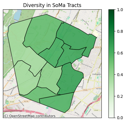
Plot the Maps
Now we can plot diversity and integration as heat maps. We did just some very basic styling on these plots, but of course you can do whatever you want to make them the best visualizions for your purposes.
[15]:
ax = cem.plot_map(
    gdf_essex_di,
    "diversity",
    cmap="Greens",
    edgecolor="black",
    alpha=0.9,
    with_background=True,
    legend=True,
    vmin=0.0,
    vmax=1.0,
)

ax.set_title("Diversity in SoMa Tracts")

ax.tick_params(
    left=False,
    right=False,
    bottom=False,
    labelleft=False,
    labelbottom=False,
)
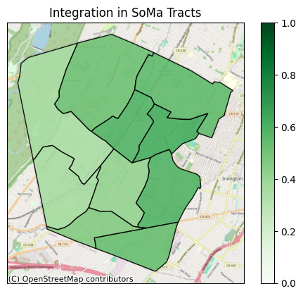
[16]:
ax = cem.plot_map(
    gdf_essex_di,
    "integration",
    cmap="Greens",
    edgecolor="black",
    alpha=0.9,
    with_background=True,
    legend=True,
    vmin=0.0,
    vmax=1.0,
)

ax.set_title("Integration in SoMa Tracts")

ax.tick_params(
    left=False,
    right=False,
    bottom=False,
    labelleft=False,
    labelbottom=False,
)
[ ]: