ACS Demo
Introduction
This notebook demonstrates how to load US Census American Community Survey (ACS) 5-year data detailed tables and do demographic analysis on it. The process is very much parallel to how we loaded and used US Census redistricting data in the SoMa DIS Demo and Seeing White notebooks.
Imports and configuration
[1]:
# So we can run from within the censusdis project and find the packages we need.
import os
import sys

sys.path.append(
    os.path.join(os.path.abspath(os.path.join(os.path.curdir, os.path.pardir)))
)
[2]:
import censusdis.data as ced
import censusdis.states

import divintseg as dis
[3]:
# Set your API key here.
CENSUS_API_KEY = None
[4]:
YEAR = 2019
DATASET = "acs/acs5"
[5]:
# Feel free to try other states.
STATE = censusdis.states.STATE_NJ
[6]:
# A group of variables counting people by race and ethnicity.
# See https://api.census.gov/data/2019/acs/acs5/groups/B03002.html
GROUP = "B03002"
Load the data and compute diversity and integration
[7]:
df_acs5 = ced.download(
    DATASET,
    YEAR,
    leaves_of_group=GROUP,
    state=STATE,
    block_group="*",
    api_key=CENSUS_API_KEY,
)
[8]:
df_di = dis.di(
    df_acs5,
    by=["STATE", "COUNTY", "TRACT"],
    over="BLOCK_GROUP",
).reset_index()

df_di.head()
[8]:
| STATE | COUNTY | TRACT | diversity | integration | |
|---|---|---|---|---|---|
| 0 | 34 | 001 | 000100 | 0.799079 | 0.742759 |
| 1 | 34 | 001 | 000200 | 0.774784 | 0.701973 |
| 2 | 34 | 001 | 000300 | 0.781342 | 0.726768 |
| 3 | 34 | 001 | 000400 | 0.765627 | 0.687127 |
| 4 | 34 | 001 | 000500 | 0.695903 | 0.685162 |
Add geography to our dataframe
[9]:
gdf_di = ced.add_inferred_geography(df_di, YEAR)
Plot the data for the state
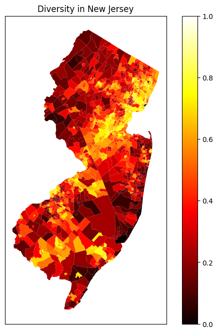
[10]:
import matplotlib.pyplot as plt

plt.rcParams["figure.figsize"] = (8, 8)

ax = gdf_di.plot(
    "diversity",
    cmap="hot",
    legend=True,
    vmin=0.0,
    vmax=1.0,
)

ax.set_title(f"Diversity in {censusdis.states.NAMES_FROM_IDS[STATE]}")

ax.tick_params(
    left=False,
    right=False,
    bottom=False,
    labelleft=False,
    labelbottom=False,
)
[ ]: